VAE: giving your Autoencoder the power of imagination

In this article we will take a detailed look at the Variational Autoencoder: a generative model that is based on its more commonplace sibling, the Autoencoder (which we will devote some time to below as well). Stay tuned for the PyTorch implementation in the next post!

Before there were GANs, there were VAEs. (And before there were VAEs, there were AEs. Do not even get me started on the VAE-GANs; let us first decipher all these acronyms before they get out of hand!)

Now let's go through them one at a time.

Autoencoder: How do you describe a face?

Autoencoder is an unsupervised machine learning algorithm, that aims to obtain a low(er) dimensional representation of your input. This might not sound like a big deal, but the idea is actually quite deep if you think about it. First of all, what is a representation? It is how you choose to describe something, in a way that works well enough for your purposes. For instance, let's say you witnessed an armed robbery committed by this lady over here:

With the incident being something out of the ordinary in your daily life, the image of the cheerful robber is deeply ingrained in your memory. On the bright side, the police is happy to hear it, and the forensic artist asks you to describe the suspect for their sketch. How would you go about it?

Even if you had the photo above at your disposal, your description probably would not start with "Well, if I was to produce a 1024 by 1024 pixel portrait of her, the value of the pixel in the lower left corner would be..." You don't actually need 1024 x 1024 numerical values to characterise someone's face – not to mention that this type of word picture does not come naturally to us, humans. Instead, you might say that she had wavy reddish hair, a round face, a medium-sized nose, and green eyes. The forensic artist would then use their knowledge of what a human face looks like plus your description to produce a sketch of the lady robber. The resulting digital sketch would indeed be made up of pixels, but that is not the representation that you and the artist used between the two of you in the process.

What is a face to a neural network?

An artificial neural network trained on people's portraits develops its own ideas on what constitutes a human face. To a computer at large, the photo above is nothing more than 1024 x 1024 (x 3 due to the three color channels per pixel) integer values. However, a trained artificial neural network can describe it using certain characteristics instead – not unlike how we would go about it. These characteristics will be encoded numerically, and can therefore be combined together to form a one-dimensional array of numbers, i.e. a vector. The vector's dimensionality will vary depending on the problem at hand, but it will generally be much lower than the dimensions of the original input: for our 1024x1024 portraits, we can probably get away with several hundred (say, 512) for most practical purposes. These 512 characteristics may (and, in all probability, will) be different from what we could imagine: e.g. assigning a certain variable to the distance between the person's eyes, another one to encode the person's skintone, etc. But they will make as much sense to the trained network, as saying "wavy reddish hair" does to us.

How do we arrive at such a description in practice? So far we have been discussing images. Although the concept of autoencoders is by no means limited to computer vision, images are probably the easiest data format to illustrate an example model architecture with. A typical image autoencoder has two parts: an encoder, consisting of several convolutional layers, and a decoder, that is comprised of deconvolutional layers. Since the input first shrinks in size as it goes through the encoder, and then expands back to its original shape inside the decoder, the outer layer of the encoder, whose output has the lowest dimensionality, is often called the bottleneck.

The two parts often are, but do not have to be, symmetric in their architecture. The encoder is a convolutional network that is trained to recognise features of the input images: the deeper the layer, the more abstract the features. What we are after is the output of the bottleneck layer – which is the neural network's description of the input. This low dimensional representation is sometimes called the latent representation (in NLP, you may also find it referred to as a context vector for a phrase).

During training, the autoencoder is supplied with images from the training set, which it is expected to recreate once they pass through the bottleneck layer. The idea is that in order to do that, what comes out of the bottleneck should contain enough information for the network to be able to generate the original image, or something close enough to it.

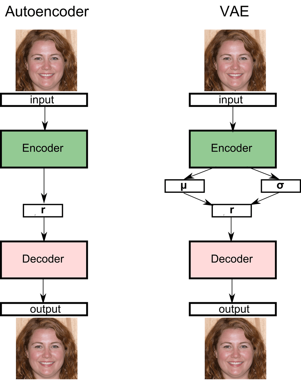
An autoencoder 1) takes an image, 2) analyses it via the convolutional encoder, 3) arrives at the latent representation of the image, and 4) generates, via the deconvolutional decoder, 5) the output image. The training objective is to minimize the difference between the input and output images.

The training objective is enforced through the use of a pixelwise loss function: typically the sum of either the absolute values of the differences, or the squares of the differences, between each pixel's ground truth value and that which has been generated by the network.

What do we use autoencoders for?

Autoencoders have a variety of applications in and out of the computer vision field. The most obvious one is the data compression mechanism that they provide: data can be compressed via the encoder network, and restored from its latent form via the decoder. Additionally, since the goal of the autoencoder is to learn the most "useful" features of the data, it can also serve to remove noise from the inputs. To facilitate training for this task, we can add synthetic noise to the inputs that are fed into the encoder, and compare the decoded outputs to the original noise-free images. (The same approach can be applied to the problem of image colorisation for instance – although at that point, it would not make much sense to refer to your model as an autoencoder.)

Autoencoder is a widely used unsupervised machine learning algorithm. Speaking of unsupervised learning, another popular unsupervised approach is clustering. Just as the name would suggest, clustering amounts to assigning datapoints that share certain characteristics (i.e. are located close to each other in feature space) into groups. However, the higher the number of dimensions of the said feature space, the more difficult it is to do clustering. This is where an autoencoder can come in handy as a dimensionality reduction technique: first the data is used to train an autoencoder, then the autoencoder is employed to encode the data into a low(er) dimensional latent space, and finally, a clustering algorithm is run on the encoded datapoints.

Another application of autoencoders is anomaly detection. Generally autoencoders are trained on samples that share something in common: e.g. in our example above, the training samples were images of people. A well-trained autoencoder should then be able to reproduce a (previously unseen) input up to a small error. (Here the definition of small depends on the equally vague notion of well-trained.) Let us say that you trained an autoencoder on data from a certain domain, and now you get some new data. You want to know whether these new data come from the same domain. You can do this by computing the losses for the new data samples: whatever gives rise to a much greater reconstruction loss than the others, gets labeled as an anomaly.

Variational Autoencoder

A variational autoencoder is a generative model: meaning, it learns from the data that we supply it with, and then generates new data (typically using random noise vectors as inputs) that look like the training data. For instance, a VAE trained on MNIST will produce brand new images that look like handwritten digits.

In a "vanilla" autoencoder from the previous section, the decoder generates restored images from the latent vectors that it encodes the training images into. In principle, we can treat the decoder as a separate neural network that simply takes vectors of a certain dimensionality as inputs (e.g. in the face autoencoder example above, we agreed to set this dimensionality to 512). What happens if, instead of encoding an existing image as a latent vector, we choose a random 512-dimensional vector and feed it through the decoder? Well, generally speaking, nothing much. You would likely get a rather noisy output that would look nothing like the domain whose data you have been working with. Can we do better? Let us ask VAEs.

The crucial difference between a vanilla autoencoder and the variational one is that a VAE learns a (typically, normal) distribution for the vectors in the latent space. Here is another way of putting it: there are many different ways for images to be encoded into and decoded from the latent space. However, this does not mean that an arbitrary vector that lies, say, in between two such latent representations can be decoded into a sensible output image. In order to pull that off, out of all the ways there are to encode our images, we need to choose one that has some nice properties. An excellent mathematical-enough-yet-intuitive explanation as to what those nice properties are is provided in this blogpost.

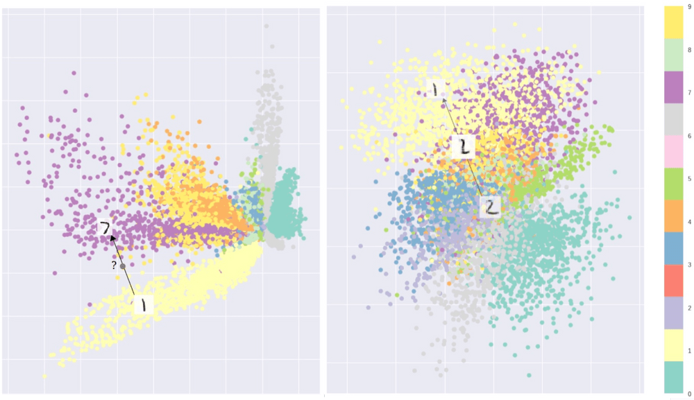
In the figure below, taken from Intuitively Understanding Variational Autoencoders, you will find an example of the autoencoder+clustering application that we discussed above. Here MNIST images of hand-written digits have been encoded in the two-dimensional space, allowing us to plot them as points on the plane. Naturally, there are many embeddings that will do the job, and two such examples are shown below:

Image source: Towards Data Science

In both cases, points of different colors (i.e. images corresponding to different classes) have a clear tendency to form clusters. However, consider the following. Do you ever have trouble distinguishing 1 and 7? We've all been there, especially when it comes to a North American 7 (the one without the dash through the middle) vs. a European 1 (with a little beret on top). One would think that interpolating between these two digits would be trivial then, but that is not the case for a generic autoencoder. Look at the plot on the left in the figure above: the purple points (the "sevens") and the lime yellow ones (the "ones") are separated by an empty space. So if you choose a point in between the two and feed it as input to your decoder, the model will not know what to do with it! However, you can force the latent space in which your two-dimensional MNIST embeddings live to have a much more regularized structure – such as the one on the right. Here you can select a pretty much arbitrary point within the multi-colored MNIST "blob" and the decoder will generate something MNIST-like: either a digit that can be clearly recognized as such, or at least an image with digit-like features. For an arbitrary input, the output image will not be sourced from the training set, rather it will be generated from scratch (well, technically from a two-dimensional input vector, but you see what I mean).

Such a structure of the latent space is achieved through a combination of encoding the training samples as distributions rather than vectors, and introducing what is called the Kullback-Leibler divergence in addition to the standard autoencoder term in the loss function. (Kullback–Leibler divergence is what forces the distribution of the latent representations to resemble a Gaussian.) Mathematics aside, let us see what actually happens during the VAE training:

1. First, the training sample gets encoded as a distribution over the latent space. That is to say, that instead of a single vector r1 (r for representation), we get two vectors: μ1 and σ1 (where μ and σ correspond to the mean and the standard deviation for the distribution). To put it less mathematically, instead of being mapped into a point in the l-dimensional latent space, the input gets mapped into a fuzzy l-dimensional sphere.
2. Then, a vector (which we might as well call r1) gets sampled from the distribution we arrived at in the previous step. In other words, a particular point gets picked out from that fuzzy sphere we've got.
3. From then on, we proceed just as we would have with a regular, non-variational autoencoder: put r1 through the decoder, generating an output image, and compute the reconstruction error (pixelwise difference between the input image and the generated output). Afterwards we can backpropagate the computed gradients through the network and updated its parameters accordingly.

The architecture of the VAE actually closely resembles that of the Autoencoder, with the main difference being that the input is encoded into two vectors, rather than one. These two vectors are used to define a normal distribution, where the latent representation of the input is then drawn from.

Each of the three steps above is rather straightforward, but there is one subtlety that is easy to miss. In step two we sample a vector from the distribution that our input was encoded into. This is, of course, something we can do, there is even a method in torch that we can use for this operation. torch.normal takes a mean and a standard deviation and returns a mean-shaped tensor drawn from the corresponding distribution. However, there is one problem: how do we run backpropagation through a node like that? Backpropagation through a sampling operation is not defined. In order to get around this problem, we are going to make use of the following reparametrization trick: set r1 equal to μ1 + σ1* ε where the stochastic part comes from ε,a vector drawn from a normal distribution with mean 0 and variance 1, eps = torch.randn_like(mean). Now that we have divided the sampling operation into a stochastic part (where the sampling actually takes place) and a deterministic one (meaning the μ1 and σ1 vectors), we can run backpropagation through the latter and be done with it.

In the next blogpost, we are going to see how these principles can be put together and implemented in PyTorch to train a Variational Autoencoder on one of the Scaleway GPU instances, and use the trained model to generate some brand new images!